Here's what's on deck. Check Canvas for full instructions and submission links.
Two cards, twenty seconds: tap the one with the smaller water footprint. The faster you pick correctly, the more points you earn.
Three kinds of water are counted. Food and clothing: the global-average water footprint of the whole supply chain (rain and irrigation water used to grow the crop or the animal feed, plus the water needed to dilute the pollution). At home and in the yard: the water that comes out of the tap. Electricity: the water a power plant consumes while running (for coal and gas, mostly evaporated in cooling towers) to make one week of an average U.S. home’s electricity (207 kWh). 1 gallon = 3.785 liters.
| A week of wind power average U.S. home | 0.24 L (0.06 gal) | 207 kWh × about 0.3 gallons per MWh (onshore wind operations, reported as 0.1–0.5) (Meldrum et al. 2013; EIA) |
| A week of solar power average U.S. home | 0.78 L (0.21 gal) | 207 kWh × 1 gallon per MWh (utility PV, mostly panel washing) (Macknick et al. 2012; EIA) |
| Flushing a toilet one flush, federal‑standard toilet | 6.1 L (1.6 gal) | 1.6 gallons per flush, the federal maximum (a WaterSense-labeled toilet uses 1.28 or less) (EPA WaterSense (federal standard)) |
| Running an ENERGY STAR dishwasher one full load | 12 L (3.2 gal) | 3.2 gallons per cycle, the ENERGY STAR limit (ENERGY STAR) |
| A load of laundry standard washing machine | 76 L (20 gal) | 20 gallons per load for a standard machine (ENERGY STAR) |
| A 10‑minute shower federal‑standard showerhead | 95 L (25 gal) | 10 minutes × 2.5 gallons per minute, the federal maximum (a WaterSense-labeled head uses 2.0 or less) (EPA WaterSense (federal standard)) |
| Washing a load of dishes by hand 12 place settings | 103 L (27 gal) | 103 liters, the European average measured for 12 place settings (country averages run 35–160 liters) (Stamminger et al.; Berkholz et al. 2013) |
| A cup of coffee 125 mL, 7 g of coffee | 130 L (34 gal) | 18,900 liters per kg of roasted coffee × 7 g = 130 liters (Water Footprint Network; Mekonnen & Hoekstra 2011) |
| A pound of potatoes fresh | 130 L (34 gal) | 287 liters per kg × 1 lb (Mekonnen & Hoekstra 2011; Water Footprint Network) |
| Drip‑watering a 100 ft² garden same plant need as 1 inch by sprinkler | 153 L (41 gal) | a 1-inch sprinkler watering of 100 ft² is 62 gallons; drip meets the same plant need with about 35% less (midpoint of EPA’s 20–50%), applying about 0.65 inch (EPA WaterSense; USGS) |
| A week of natural gas power average U.S. home | 161 L (42 gal) | 207 kWh × 205 gallons per MWh (combined cycle, cooling tower) (Macknick et al. 2012; EIA) |
| One egg 60 grams | 196 L (52 gal) | 196 liters for a 60-gram egg (Mekonnen & Hoekstra 2012; Water Footprint Network) |
| A week of coal power average U.S. home | 538 L (142 gal) | 207 kWh × 687 gallons per MWh (coal, cooling tower) (Macknick et al. 2012; EIA) |
| A chocolate bar 100 grams | 1,700 L (449 gal) | about 17,000 liters per kg × 100 g = 1,700 liters (Water Footprint Network; Mekonnen & Hoekstra 2011) |
| A quarter‑pound hamburger the beef patty | 1,748 L (462 gal) | 15,415 liters per kg of beef × ¼ lb (Mekonnen & Hoekstra 2012) |
| A pound of chicken chicken meat | 1,962 L (518 gal) | 4,325 liters per kg × 1 lb (Mekonnen & Hoekstra 2012; Water Footprint Network) |
| A pound of dry beans uncooked | 2,292 L (605 gal) | 5,053 liters per kg × 1 lb (Mekonnen & Hoekstra 2011) |
| Sprinkling a 1,000 ft² lawn one inch of water | 2,360 L (623 gal) | 1 inch over 1,000 ft² (27,154 gallons per acre-inch × 1,000 ÷ 43,560) (USGS) |
| A cotton T‑shirt 250 grams of cotton | 2,500 L (660 gal) | 10,000 liters per kg of cotton fabric × 250 g (Water Footprint Network; Mekonnen & Hoekstra 2011) |
| A pound of almonds shelled | 7,301 L (1,929 gal) | 16,095 liters per kg (shelled) × 1 lb (Mekonnen & Hoekstra 2011) |
Earth holds about 332 million cubic miles of water. Almost all of it is salty; only about 2.5% is fresh, and most of that is frozen or underground.
Tap a slice or a label. Data: U.S. Geological Survey, Water Science School, “Where Is Earth’s Water?” usgs.gov/special-topics/water-science-school. Volumes from I. Shiklomanov (1993), “World Fresh Water Resources,” in P. H. Gleick (Ed.), Water in Crisis: A Guide to the World’s Fresh Water Resources, Oxford University Press.
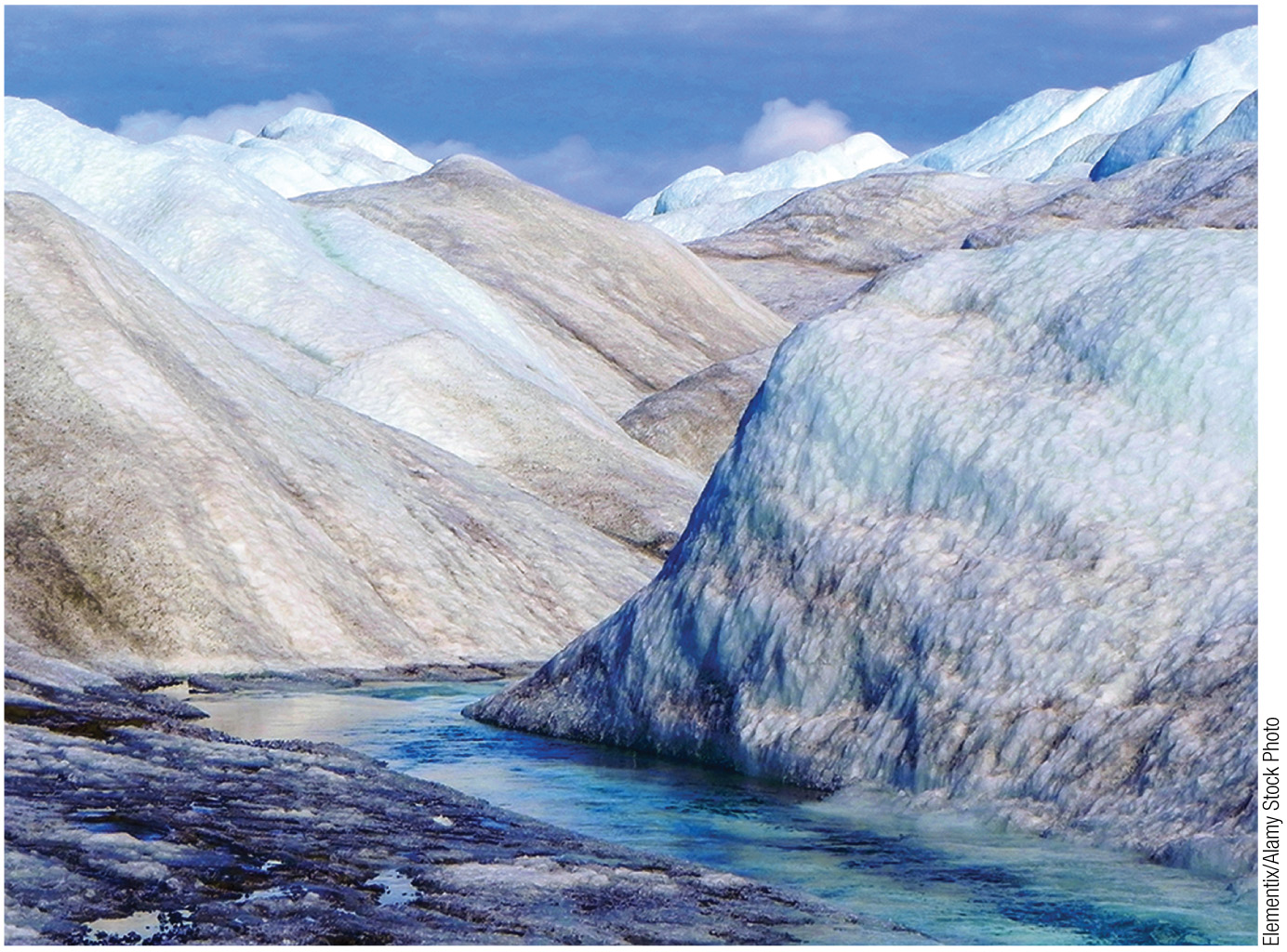
The hydrosphere is all the places on Earth that hold water. Water collects in reservoirs, where it stays for a time; the ocean is by far the largest.
USGS Water Science School, Oceans and Seas and the Water Cycle and Groundwater Flow and the Water Cycle; Mekonnen & Hoekstra (2012), Ecosystems 15 (pork: 5,988 L/kg).
Water mining means withdrawing groundwater faster than it is replenished. This excessive groundwater withdrawal can lead to aquifer depletion.
UN-Water (2022), Groundwater: Making the Invisible Visible, joint message for the UN-Water Summit on Groundwater: six-fold increase in abstraction over the last 70 years.
USGS Water Science School, Land Subsidence.
A constant supply of water and power, paid for downstream.
Dams store water through dry seasons and generate hydroelectric power, and diversions carry that water to cities and farms. The costs fall on the river below the dam and on the people and ecosystems that depend on it.
Disrupted fish migration, lost wetlands, altered sediment transport, changed river temperatures, and diminished downstream flows.
Upstream dams and diversions have so reduced its flow that it no longer consistently reaches the Gulf of California.
1 Veldkamp, T. I. E., et al. (2017). Water scarcity hotspots travel downstream due to human interventions in the 20th and 21st century. Nature Communications, 8, 15697. Colorado River: U.S. Bureau of Reclamation, Colorado River Basin Water Supply and Demand Study (2012).
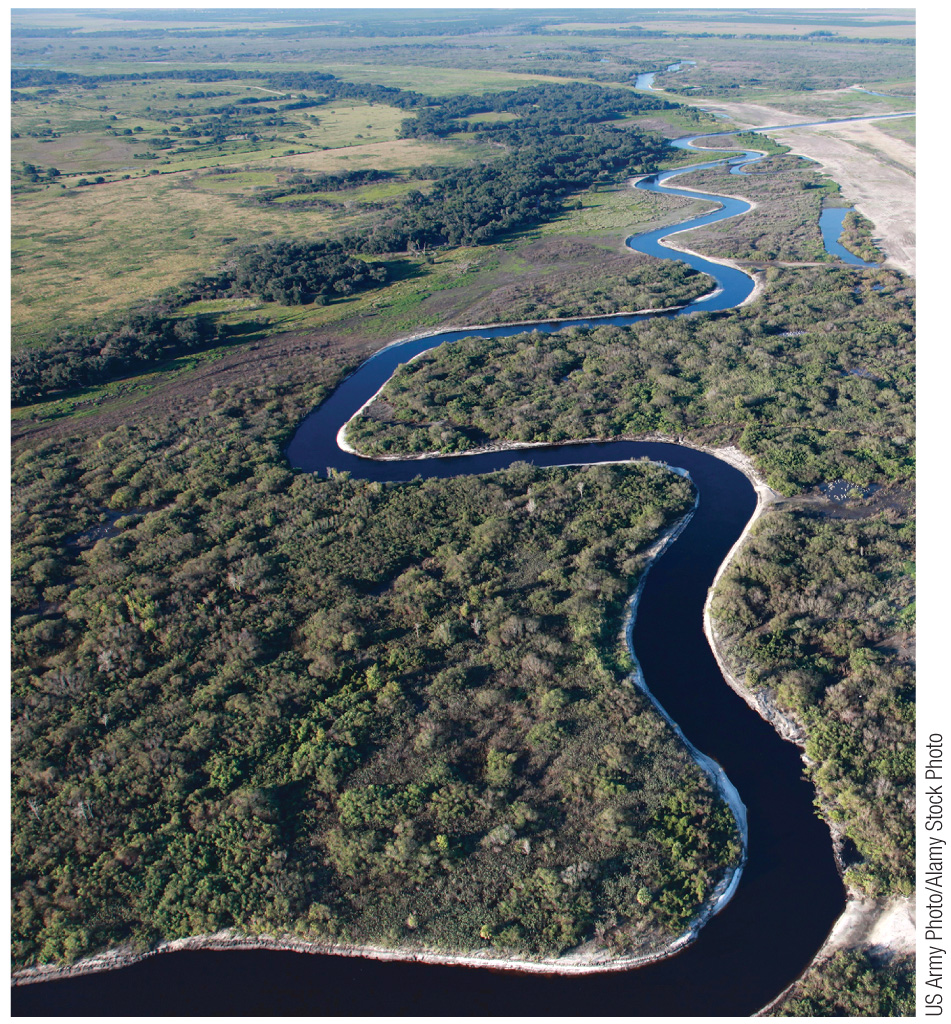
Regulation is easiest when you can point to the pipe.
Contaminants from a clearly identifiable conduit, such as a pipe, ditch, channel, or well. The source is known, so it can be permitted and monitored.
Pollutants from broad, diffuse places: agricultural, residential, and industrial activities across a whole watershed.
Loose soil swept into waterways makes the water turbid (cloudy) and reduces light penetration.
Chemicals from agriculture, energy, and infrastructure (as in Flint); bacterial and viral contamination, including feedlot runoff.
Sources: U.S. EPA, Basic Information about Nonpoint Source (NPS) Pollution and NPDES Permit Basics; USGS Water Science School, Turbidity and Water.
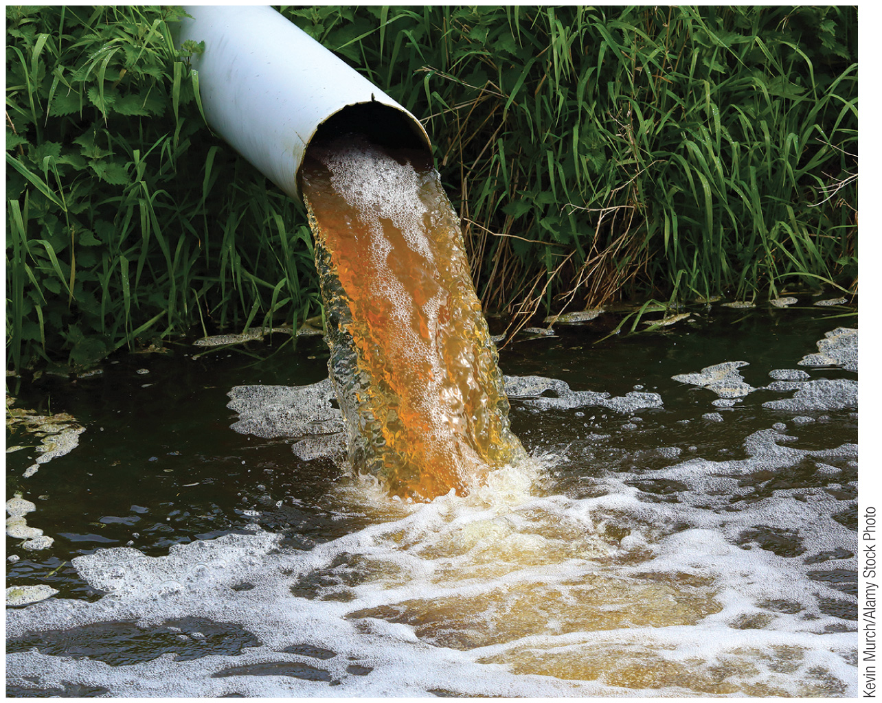
To cut costs while waiting for a new pipeline, Flint switched its water source in 2014, a decision with severe consequences.
Flint Water Advisory Task Force (2016), Final Report, Office of the Governor of Michigan; U.S. EPA Office of Inspector General (2018), Report 18-P-0221.
Too much of a good thing: how fertilizer can starve a lake of oxygen.
Excess fertilizer runoff leads to increased levels of nitrogen and phosphorus, which fuel algae growth and, as the algae die and decay, oxygen depletion in the water.Sources: U.S. EPA, Nutrient Pollution; NOAA National Ocean Service, What Is Eutrophication?
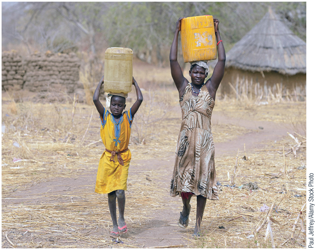
The UN's goal of water security means reliable access to safe, affordable water for everyone.
WHO/UNICEF JMP (2025), Progress on Household Drinking Water, Sanitation and Hygiene 2000–2024; California EO B-29-15 (2015); City of Cape Town, Water Outlook 2018. Photo: Paul Jeffrey/Alamy Stock Photo, via W. W. Norton.
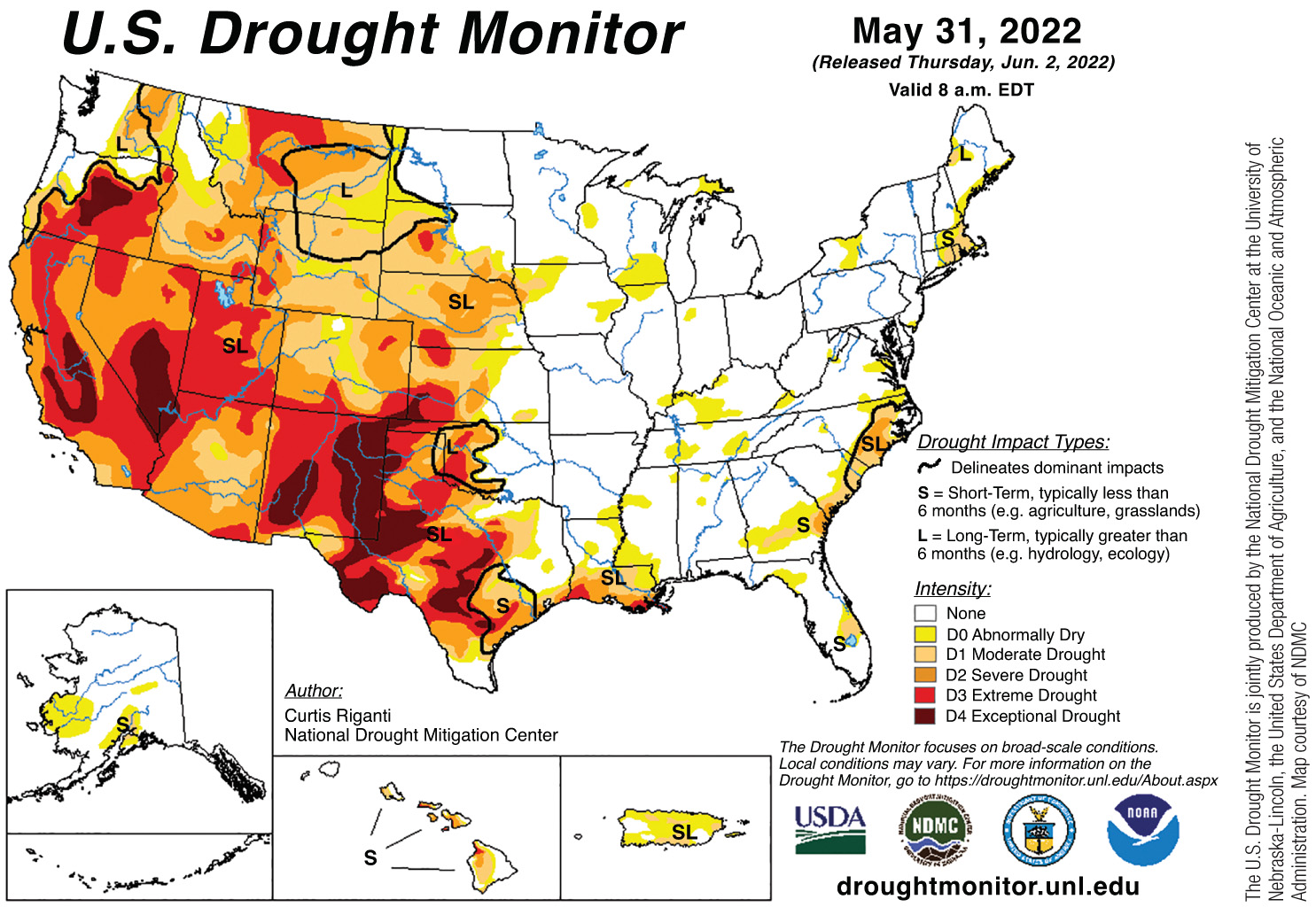
Map: U.S. Drought Monitor, May 31, 2022 (National Drought Mitigation Center, USDA, NOAA), as reproduced in Sherman & Montgomery (2023), W. W. Norton.
U.S. EPA WaterSense, Microirrigation and Outdoor Water Use in the United States; ADWR, Conservation programs.
U.S. EPA, Nonpoint Source: Agriculture.
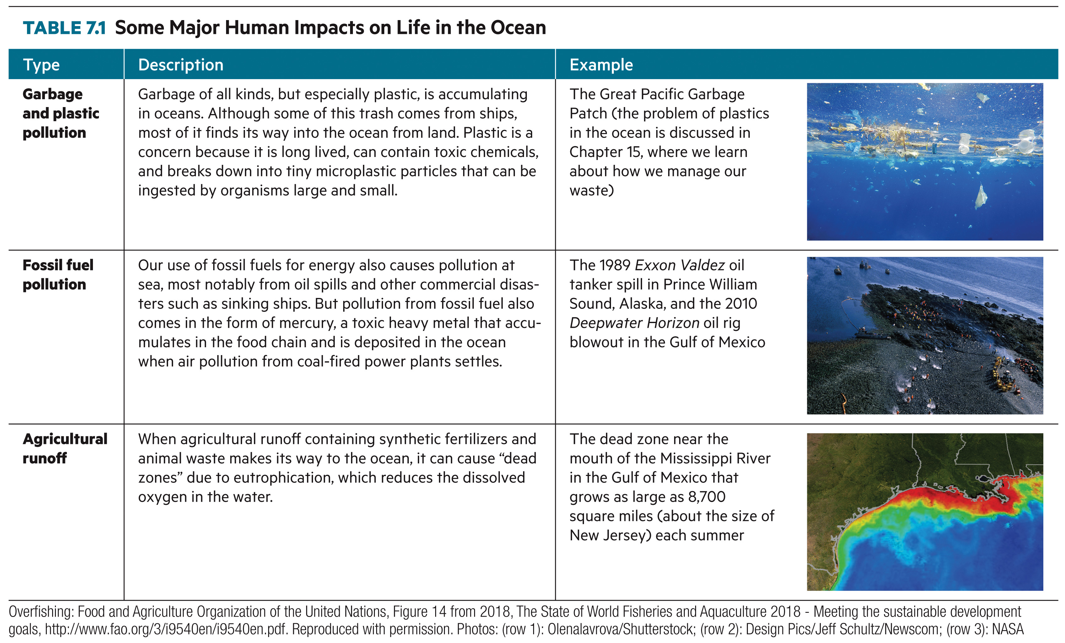
Human activity harms the ocean in three big ways: plastic garbage that breaks into microplastics, which can carry and release harmful chemicals; fossil-fuel pollution from spills and airborne mercury; and agricultural runoff that creates oxygen-starved “dead zones.”
NOAA Marine Debris Program, Microplastics; NOAA, Gulf of Mexico Dead Zone. Table 7.1 from Sherman & Montgomery (2023), W. W. Norton; photos: Olenalavrova/Shutterstock, Design Pics/Jeff Schultz/Newscom, NASA.
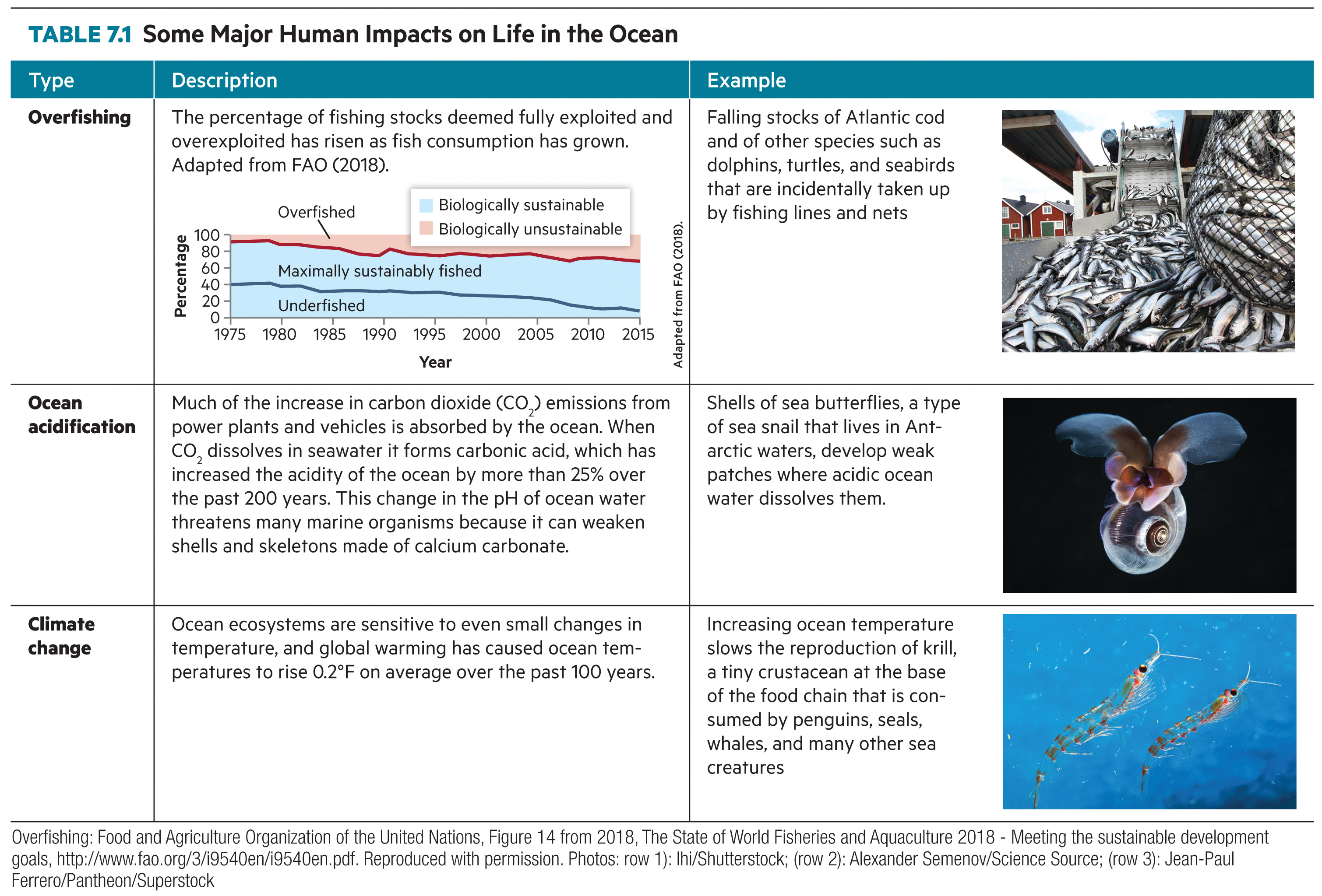
Three more pressures push ocean ecosystems toward collapse: overfishing faster than stocks can recover, a warming climate that disrupts food webs, and acidification. As the ocean absorbs CO₂, its pH falls and carbonate ions grow scarcer, so shell-building animals struggle to build and keep their calcium carbonate shells.
NOAA Pacific Marine Environmental Laboratory, What Is Ocean Acidification?; FAO (2018), The State of World Fisheries and Aquaculture. Table 7.1 from Sherman & Montgomery (2023), W. W. Norton; photos: Ihi/Shutterstock, Alexander Semenov/Science Source, Jean-Paul Ferrero/Pantheon/Superstock.
ASU’s Global Futures Water Institute is “dedicated to forecasting and tackling water challenges at all scales, from local communities to national systems.” In the desert Southwest, individual choices add up. Here’s where to start.
Spend your policy budget, zone your city on the river, and decide how fast it grows. Then thirty years arrive, one at a time.
| Parameter | Value | Status | Basis |
|---|---|---|---|
| Houses: water per square | 188 AF/yr (480 homes) | Derived | Multi-City Water Use Study: about 350 gal/day per single-family home, 57% outdoors |
| Apartments: water per square | 652 AF/yr (3,200 units) | Derived | Water Research Foundation: 182 gal/day per Phoenix multifamily unit |
| Shops & offices, industry: water | 150 and 640 AF/yr | Assumed | Teaching values scaled to typical commercial and industrial use |
| Alfalfa, vegetables, orchards | 864, 624, 720 AF/yr (160 acres) | Derived | Univ. of Arizona (2023), Table C1: 5.4, about 3.9, about 4.5 AF per acre |
| Dairy | 235 AF/yr (2,000 cows) | Derived | ADWR allotment: 105 gal per cow per day |
| Green park turf | 368 AF/yr | Derived | ADWR turf allotment 4.6 AF/acre on half the square |
| Farm output | $0.4M to $12M per square | Derived | USDA NASS Arizona prices and yields (2022) |
| Construction income, output per job | NAHB per-home values; $120,000 per job | Derived | NAHB (2015); BEA/BLS Phoenix metro (2022) |
| Residential price elasticity | −0.41 | Measured | Dalhuisen et al. (2003) meta-analysis |
| Pumping cost | about $0.20 per AF per foot of lift | Derived | Hanson (UC ANR) energy per lift, at about $0.10/kWh |
| Incidental recharge | 25% of farm water, 4% of city water | Measured | ADWR Phoenix AMA groundwater model (2024) |
| River: normal flow and each city’s share | 5,500 AF per city | Assumed | Every city holds an equal share, set so a normal year exactly covers the class; dry years cut every city |
| Wet and dry years | 4-state Markov chain, 58% to 128% of normal | Assumed | Stylized; clustered like real river flows |
| Megadrought | 22 years near 52% of normal | Assumed | Shaped on Williams, Cook & Smerdon (2022), not a reconstruction |
| Aquifer | 60,000 AF usable; 1,800 AF/yr recharge; fossil ×0.2, fast ×1.7 | Assumed | Teaching values |
| Subsidence | below 20% of the aquifer; capacity drops to 70% | Assumed | Direction from USGS subsidence studies; sizes assumed |
| Confidence, moving away, sprawl, drilling | rates in the code; while taps run, a falling aquifer drives away 35% as many people as it deters investment; Managed and Steady cities pause building below 85% and 65% of the aquifer and set water rules below 80% (outdoor watering and farmland cut up to 40% Managed, 25% Steady) while the wells outpace recharge | Assumed | Stylized behavioral rules, not estimated |
| Eutrophication | algae past about three riverbank farms’ runoff (two with a dairy); a farm two squares from the river sends 50%, three squares 25%, farther 12%; a buffer square beside a farm traps 45% of its runoff (two squares away, 25%); a buffer-lined riverbank traps up to 60% more; buffer law traps 50% | Assumed | Direction from Mayer et al. (2007); sizes assumed |
| Policy effects | conservation −30% outdoor, −10% indoor; recycling 3,000 AF; permits ×1.8; tax ×1.2; chip plant ×2 output, ×1.6 water; farm exports ×1.4 farm output, ×1.2 farm water; job training ×1.15 job output | Assumed | Teaching values in plausible ranges |
| Chip plant cost | $9M a year | Assumed | Scaled down for a small city from Phoenix’s $205M TSMC infrastructure package (2020), which annualizes to about $13M a year |
| Policy budget | $10M a year per city | Assumed | Set so a city can afford a few policies, not all of them |
| Build-now budget | $500M, up to 6 squares, standing from year 0 | Assumed | Set so a student can build a handful of squares before zoning |
| Cost to build a square | houses $138M, apartments $374M, shops $77M, industry $120M; farms and parks $3M to $14M | Derived | Homes and businesses: the construction values above (NAHB); farms and parks assumed |
| Other policy costs | $1.5M to $5M a year | Assumed | Rough annualized capital and program costs |
| Sustainability score | 40% renewable share, 35% aquifer left, 25% recent reliability | Assumed | A teaching index |